Balancing the nutritional status of potato crops.
2020-02-01
Chapter 1 Data processing
1.1 Objective
This chapter is the first of a series of R markdown codes aiming to describe computations methodology used to derive the results and conclusions of potato nutrient diagnosis article. The data set is a collection of potato surveys and N, P and K fertilizer trials conducted in Quebec from 1970 to 2017 between the US border at the 45^th parallel and near the Northern limit of cultivation at the 49^th parallel. The useful variables are the first mature leaf (4^th from top, collected at the beginning of blossom stage) N, P, K, Ca and Mg compositions, cultivars used in experiments and tuber marketable yield. These variables are selected from the Québec potato raw data table (raw_leaf_df.csv) and processed to give useful variables for cultivars clustering (Chapter 2), tuber yield prediction (Chapter 3) and assessment of perturbation vector concept (Chapter 4). A previous exploration showed that oligoelements contained too many missing values, for this reason these elements were excluded from analysis. The chapter ends with the backup of a processed data frame useful for next chapters.
1.2 Useful libraries for data handling
We need package tidyverse which loads a set of packages for easy data manipulation and visualization. A set of other packages is used: Amelia for missing data vizualisation, robCompositions to robustely impute missing values in compositional data using k-nearest neigbhors methods, and compositions to transforme compositions into compositionnal space.
1.3 Québec potato data set
Let’s load the Québec potato leaves raw compositions data set raw_leaf_df.csv available for the project in the data folder.
1.4 Selection of useful variables
We create custom vectors of attributes which help select useful data columns for computations. The year of experiment is not needed instead it permits to know how long ago expériements have been monitored. Geographical coordinates are useful to map experimental sites locations later.
keys_col <- c('NoEssai', 'NoBloc', 'NoTraitement')
location <- c('Annee', 'LatDD', 'LonDD')
cultivars <- c('AnalyseFoliaireStade', 'Cultivar', 'Maturity5')
discard_col <- c("AnalyseFoliaireC", "AnalyseFoliaireS", "AnalyseFoliaireB", "AnalyseFoliaireCu",
                "AnalyseFoliaireZn", "AnalyseFoliaireMn", "AnalyseFoliaireFe", "AnalyseFoliaireAl")
longNameMacro <- c("AnalyseFoliaireN","AnalyseFoliaireP","AnalyseFoliaireK",
                   "AnalyseFoliaireCa","AnalyseFoliaireMg")
outputs <- c('RendVendable', 'RendPetit', 'RendMoy', 'RendGros')
macroElements <- c("N", "P", "K", "Ca", "Mg") # for simplicity
The reduced data frame becomes leaf_df which stands for the diagnostic leaves macroelements composition data frame combining corresponding cultivars names, marketable yield, year of experiment and sites geographical coordinates.
leaf_df <- raw_leaf_df %>% select(-discard_col)
colnames(leaf_df)[which(names(leaf_df) %in% longNameMacro)] <- macroElements
glimpse(leaf_df)
## Observations: 12,991
## Variables: 18
## $ NoEssai <dbl> 1, 1, 1, 1, 1, 1, 1, 1, 1, 1, 1, 1, 1, 1,...
## $ NoBloc <dbl> 1, 1, 1, 1, 1, 1, 1, 1, 2, 2, 2, 2, 2, 2,...
## $ NoTraitement <dbl> 1, 2, 3, 4, 5, 6, 7, 8, 1, 2, 3, 4, 5, 6,...
## $ Annee <dbl> 2003, 2003, 2003, 2003, 2003, 2003, 2003,...
## $ LatDD <dbl> 46.75306, 46.75306, 46.75306, 46.75306, 4...
## $ LonDD <dbl> -72.33861, -72.33861, -72.33861, -72.3386...
## $ AnalyseFoliaireStade <chr> "10% fleur", "10% fleur", "10% fleur", "1...
## $ Cultivar <chr> "Goldrush", "Goldrush", "Goldrush", "Gold...
## $ Maturity5 <chr> "mid-season", "mid-season", "mid-season",...
## $ N <dbl> 3.805, 3.356, 3.657, 3.610, 4.983, 4.277,...
## $ P <dbl> 0.22, 0.20, 0.22, 0.18, 0.22, 0.21, 0.28,...
## $ K <dbl> 6.31, 6.85, 6.44, 5.36, 5.92, 6.73, 5.75,...
## $ Ca <dbl> 1.69, 1.31, 1.13, 1.30, 1.23, 1.38, 1.17,...
## $ Mg <dbl> 0.53, 0.21, 0.32, 0.50, 0.44, 0.45, 0.51,...
## $ RendVendable <dbl> 18.9442, 40.3518, 33.0379, 37.5505, 46.00...
## $ RendPetit <dbl> 3.9458, 4.9159, 6.3220, 3.6515, 4.6652, 4...
## $ RendMoy <dbl> 11.4123, 17.5599, 13.6795, 16.2410, 18.99...
## $ RendGros <dbl> 3.5861, 17.8760, 13.0364, 17.6580, 22.345...1.5 Arranging the data frame
These chunks set trial number NoEssai as factor, relevel categorical maturity order variable and choose cultivar Superior as reference as it has the maximum number of observations. Then, abundance of cultivars is ploted.
percentage <- round(with(leaf_df, prop.table(table(Cultivar)) * 100), 2)
distribution <- with(leaf_df, cbind(numbOfsamples = table(Cultivar), percentage = percentage))
distribution <- data.frame(cbind(distribution, rownames(distribution)))
colnames(distribution)[3] <- "Cultivar"
distribution$numbOfsamples <- as.numeric(as.character(distribution$numbOfsamples))
distribution$percentage <- as.numeric(as.character(distribution$percentage))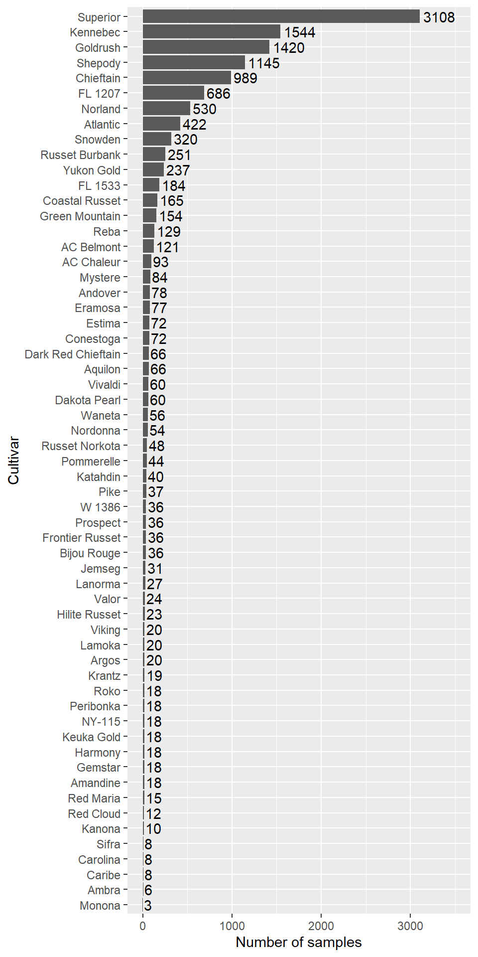
Figure 1.1: Repported cultivars abundance in the potato data frame.
leaf_df$NoEssai <- as.factor(leaf_df$NoEssai)
leaf_df$Cultivar <-  relevel(factor(leaf_df$Cultivar), ref = "Superior")
leaf_df$Maturity5 <- ordered(leaf_df$Maturity5,
                            levels = c("early","early mid-season",
                                       "mid-season","mid-season late","late"))
We portray missing values for the sake of imputation. As explained in the section ??, we will retain after this processing only reasonably imputable data i.e. samples with a number of missing variable values less than half the number of studied attributes. The next cell maps the portrait of missing values.
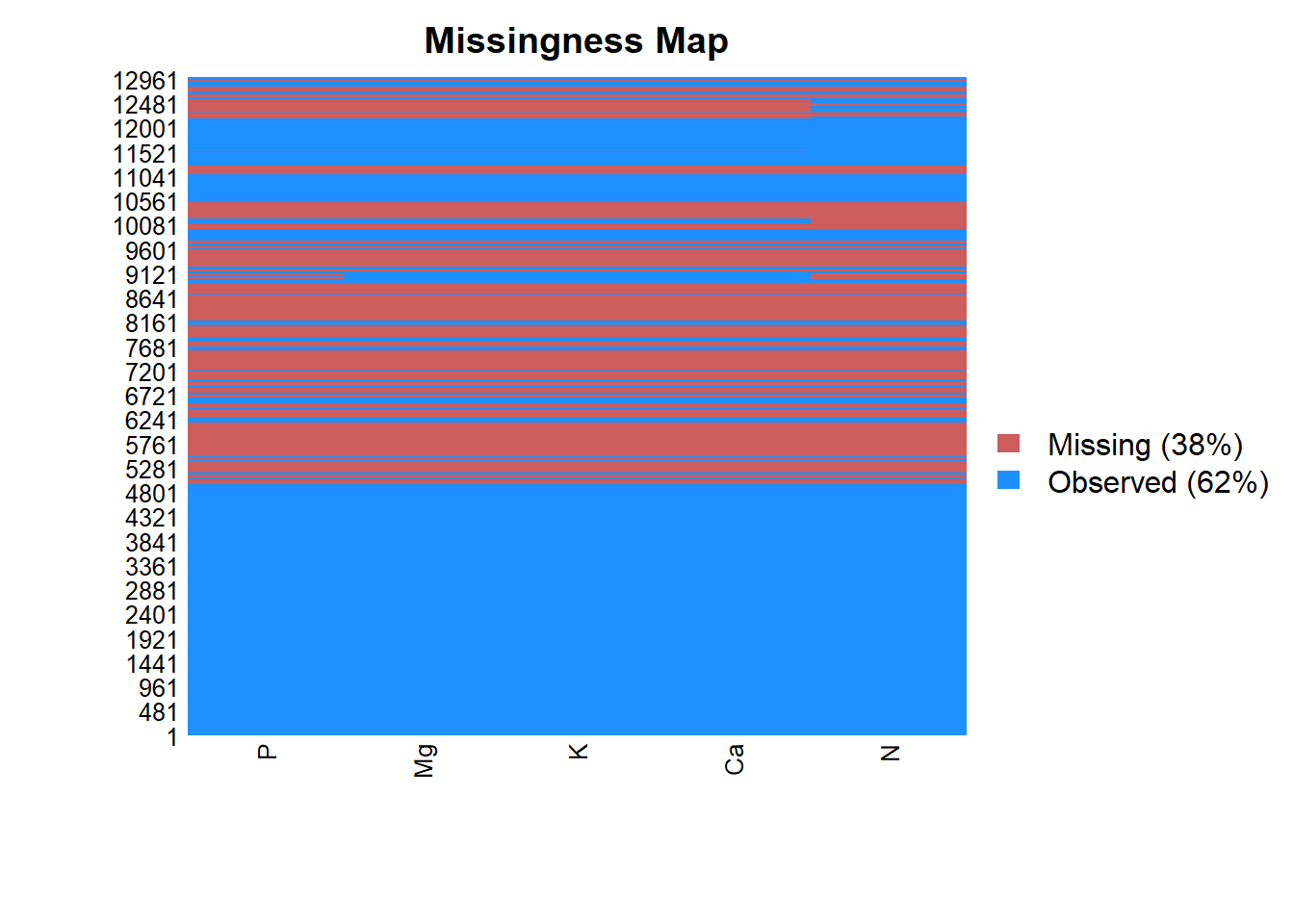
Figure 1.2: Portrait of missing macroelements.
This figure compiles the samples identifiers on the Y axis and macroelements on the X axis. A complete horizontal unique color band indicates wether the 5 elements are totally observed (blue band) or totally missing (red band). Only N and P have missing values that will be imputed and retained at the end. The totally missing compositions will be removed. The next cell initializes this process.
# keep track of empty rows:
leaf_df$leaf_allNA <- apply(leaf_df[macroElements], 1, function(X) all(is.na(X)))
# keep track of rows where there is any NA:
leaf_df$leaf_anyNA <- apply(leaf_df[macroElements], 1, function(X) any(is.na(X)))
# number of NAs (missing values):
leaf_df$leaf_countNA <- apply(leaf_df[macroElements], 1, function(X) sum(is.na(X)))
The next cell performs the imputation. Since the imputation is a time-consuming process, we saved it in a csv stored in the subfolder output and have put a switch to put on if one wants to perform the computation again. The imputation is made by KNNs in the Aitchison (compositions-friendly) metric for rows where there are 1 or 2 missing values, i.e. filter(leaf_countNA <= 3).
# Warning: could be a long process
perform_imputation <- FALSE # set to FALSE if you want to load the saved file
if (perform_imputation) {
  set.seed(628125)
  leaf_imp <- leaf_df %>%
    filter(leaf_countNA <= 3) %>%
    select(macroElements) %>%
    impKNNa(as.matrix(.),
            metric = "Aitchison",
            k = 6,
            primitive = TRUE,
            normknn = TRUE,
            adj = 'median')
  leaf_complete <- leaf_df %>%
    select(macroElements)
  leaf_complete[leaf_df$leaf_countNA <= 3, ] <- leaf_imp$xImp
  names(leaf_complete) <- paste0(names(leaf_complete), "_imp")
  write_csv(leaf_complete, "output/leaf_complete.csv")
} else {
  leaf_complete <- read_csv("output/leaf_complete.csv")
}
## Parsed with column specification:
## cols(
## N_imp = col_double(),
## P_imp = col_double(),
## K_imp = col_double(),
## Ca_imp = col_double(),
## Mg_imp = col_double()
## )With the next cell, imputed columnsare appended to the data frame. The nutrients diagnosis will be done with imputed compositions.
leaf_df <- bind_cols(leaf_df, leaf_complete)
leaf_df <- leaf_df %>% select(-c("leaf_allNA", "leaf_anyNA"))
Compositional data are data where the elements of the composition are non-negative and sum to unity. I compute Fv standing for filling value, an amalgamation of all other elements closing the simplex proportions to 100%.
leaf_df <- leaf_df %>%
  mutate(sum_imp = rowSums(select(., paste0(macroElements, "_imp"))),
         Fv_imp = 100 - sum_imp) %>%
  select(-sum_imp)
if (!"Fv" %in% macroElements) macroElements <- c(macroElements, "Fv")
The centered log-ratio (clr) transformed compositions will be used for discriminant analysis and perturbation vector concept assessment.The next cell performs this calculation. The clr coordinates are computed in an external (intermediate) data table.
leaf_composition <- leaf_df %>%
  select(paste0(macroElements, "_imp")) %>%
  acomp(.)
leaf_clr <- clr(leaf_composition) %>%
  unclass() %>%
  as_tibble()
names(leaf_clr) <- paste0("clr_", macroElements)
write_csv(leaf_clr, "output/leaf_clr.csv")
The next cell binds these clr-transformed compositions to the raw composition data frame and retains useful columns. This cell also discards all the samples with too many missing compositions.
1.6 Cultivar classes correction
From a preliminary checking, we noticed that cultivars Mystere and Vivaldi have different repported maturity classes in the data set, mid-season late and late for Mystere, then early mid-season and mid-season for Vivaldi respectively. Their new maturity classes names are based on a majority vote for this study. The next cell perform this correction. We also make missing values explicit for this categorical variable.
1.7 Summarise and backup
Finally, we summarized the processed data frame to record the years of begining and ending of experiments, the remaining number of experiments, cultivars and maturity classes. The definitive leaves data frame is stored as leaf_clust_df.csv in output subfolder as it is an intermediate file, for cluster analysis (Chapter 2).
leaf_df %>%
  summarise(start_year = min(Annee, na.rm = TRUE),
            end_year = max(Annee, na.rm = TRUE),
            numb_trials = n_distinct(NoEssai, na.rm = TRUE),
            numb_cultivars = n_distinct(Cultivar, na.rm = TRUE),
            numb_maturityClasses = n_distinct(Maturity5, na.rm = TRUE))
## # A tibble: 1 x 5
## start_year end_year numb_trials numb_cultivars numb_maturityClasses
## <dbl> <dbl> <int> <int> <int>
## 1 1970 2017 4714 59 5