Chapter 3 Predicting tuber yield category
3.1 Objective
The objective of this chapter is to develop, evaluate and compare the performance of some machine learning algorithms (k-nearest neighbors, random forest and support vector machine - package caret) in predicting tuber yield categories using clr coordinates. We use the previous chapter (chapter 2) tidded data file dfml.csv which contains clr coordinates, maturity classes and the yield two categorical variable created using the 65^th percentile for each cultivar. We use accuracy as models quality meeasure. We run a Chi-square homogenity test to compare the best model (with highest accuracy) with a random classifier consisting of an equal distribution of 50% successful and 50% unsuccessful cases.
We finally compute Euclidean distance as the measure of the multivariate distance between an observation and the closest true negative. By true negative or nutritionally balanced specimens, we mean the samples correctely predicted by the best model as high yielders in the training set. The training and testing sets are stored for the next chapter (preturbation concept - Chapter 4).
3.2 Useful libraries
The tidyverse package is always needed for data easy manipulation and visualization, and then extrafont to make changes in graphs as demanded for the article. The particularly useful packages are caret and kknn needed for machine leraning functions.
3.3 Machine learning data set
Let’s load the dfml.csv data set. The clr coordinates are scaled to zero mean and unity variance.
## Parsed with column specification:
## cols(
##   NoEssai = col_double(),
##   NoBloc = col_double(),
##   NoTraitement = col_double(),
##   clr_N = col_double(),
##   clr_P = col_double(),
##   clr_K = col_double(),
##   clr_Ca = col_double(),
##   clr_Mg = col_double(),
##   clr_Fv = col_double(),
##   RendVendable = col_double(),
##   rv_cut = col_double(),
##   yieldClass = col_character(),
##   Maturity5 = col_character(),
##   Cultivar = col_character()
## )3.4 Machine learning
3.4.1 Data train and test splits
We randomly split the data into a training set (75% of the data) used to fit the models, and a testing set (remaining 25%) used for models’ evaluation.
set.seed(8539)
split_index <- createDataPartition(dfml.sc$yieldClass, group = "Cultivar",
                                   p = 0.75, list = FALSE, times = 1)
train_df <- dfml.sc[split_index, ]
test_df <- dfml.sc[-split_index, ]
ml_col <- c(clr_no, "yieldClass")
With the kknn package, we must specify three parameters: kmax which is the number of neighbors to consider, distance a distance parameter to specify (1 for the Mahattan distance and 2 for the Euclidean distance), and a kernel which is a function to measure the distance. A best method currently used to choose the right parameters consists in creating a parameter grid.
(grid <-  expand.grid(kmax = c(7,9,12,15), distance = 1:2,
                      kernel = c("rectangular", "gaussian", "optimal")))
## kmax distance kernel
## 1 7 1 rectangular
## 2 9 1 rectangular
## 3 12 1 rectangular
## 4 15 1 rectangular
## 5 7 2 rectangular
## 6 9 2 rectangular
## 7 12 2 rectangular
## 8 15 2 rectangular
## 9 7 1 gaussian
## 10 9 1 gaussian
## 11 12 1 gaussian
## 12 15 1 gaussian
## 13 7 2 gaussian
## 14 9 2 gaussian
## 15 12 2 gaussian
## 16 15 2 gaussian
## 17 7 1 optimal
## 18 9 1 optimal
## 19 12 1 optimal
## 20 15 1 optimal
## 21 7 2 optimal
## 22 9 2 optimal
## 23 12 2 optimal
## 24 15 2 optimalThe metric of “Accuracy” is used to evaluate models quality. This is the ratio of the number of correctly predicted instances divided by the total number of instances in the dataset (e.g. 95% accurate).
The accuracy of the models will be estimated using a 10-fold cross-validation (cv) scheme. This will split the data set into 10 subsets of equal size. The models are built 10 times, each time leaving out one of the subsets from training and use it as the test set.
3.4.2 Building the Models
We reset the random number seed before each run to ensure that the evaluation of each algorithm is performed using exactly the same data splits. It ensures the results are directly comparable Jason Brownlee.
# a) Non-linear algorithm
## kNN
set.seed(7)
kknn_ <- train(yieldClass ~., data = train_df %>% select(ml_col), method = "kknn",
metric = metric, trControl = control, tuneGrid = grid)3.4.3 Goodness of fit on training set
We assess the accuracy metric also during modeling (with train set) but the target metric is for the evaluation set. This chart sorts models.
# Summary results
results <- resamples(list(kknn_model = kknn_,
                          svm_model = svm_,
                          rf_model = rf_))
#summary(results) with dotplot()
dotplot(results)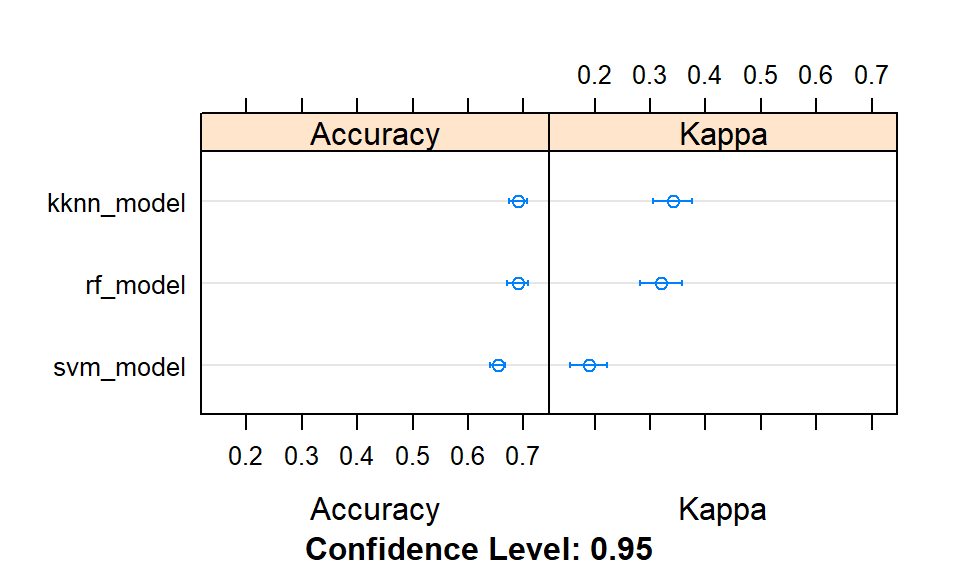
Figure 3.1: Comparison of models accuracies at training.
This chunk also sorts models in a descending order using accuracies only, in a table.
models_acc <- data.frame(Model = summary(results)$models,
                       Accuracy = c(confusionMatrix(train_df$yieldClass, predict(kknn_))$overall[1],
                                    confusionMatrix(train_df$yieldClass, predict(svm_))$overall[1],
                                    confusionMatrix(train_df$yieldClass, predict(rf_))$overall[1]))
models_acc[order(models_acc[,"Accuracy"], decreasing = TRUE), ]
## Model Accuracy
## 3 rf_model 0.9810800
## 1 kknn_model 0.8557351
## 2 svm_model 0.6748128The next one prints the best tuning parameters that maximizes model accuracy.
##        Model param.kmax param.distance param.kernel param.sigma param.C
## 1 kknn_model         12              1      optimal   0.1840573       1
## 2  svm_model         12              1      optimal   0.1840573       1
## 3   rf_model         12              1      optimal   0.1840573       1
##   param.mtry
## 1          2
## 2          2
## 3          2
3.4.4 Models’ evaluation (test set)
Model evaluation is an integral part of the model development process. It helps to find the best model that represents our data and how well the chosen model will work in the future. The next chunk performs this computations and gives the sorted accuracy metrics.
predicted_kknn_ <- predict(kknn_, test_df %>% select(ml_col))
predicted_svm_ <- predict(svm_, test_df %>% select(ml_col))
predicted_rf_ <- predict(rf_, test_df %>% select(ml_col))

#The best model
tests_acc <- data.frame(Model = summary(results)$models,
                        Accuracy_on_test = c(
                          confusionMatrix(test_df$yieldClass, predicted_kknn_)$overall[1],
                          confusionMatrix(test_df$yieldClass, predicted_svm_)$overall[1],
                          confusionMatrix(test_df$yieldClass, predicted_rf_)$overall[1]))
tests_acc[order(tests_acc[,"Accuracy_on_test"], decreasing = TRUE), ]
## Model Accuracy_on_test
## 3 rf_model 0.7076923
## 1 kknn_model 0.7065089
## 2 svm_model 0.6402367The k-nearest neighbours, the random forest and the support vector machine models returned similar predictive accuracies (although slightly higher for the former).
3.5 Variable importance estimation
The varImp() method is then used to estimate the variable importance, which is printed (summarized) and plotted. varImp() ranks features by importance.
## rf variable importance
##
##        Overall
## clr_N    220.4
## clr_Mg   201.3
## clr_Fv   193.3
## clr_K    190.8
## clr_Ca   185.5
## clr_P    184.4
#tiff('images/var-imp-plot.tiff')
plot(importance, cex = 1.2, cex.lab = 2, cex.axis = 2, ylab = "variable", col = "black")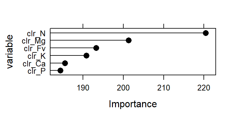
Figure 3.2: Importance of clr variables (effect) in the model.
3.6 Make predictions on the test set with kknn model
We sort the predictive quality metrics by cultivar with random forest algorithm: model rf_clr, and tide the table.
test_df$ypred = predicted_kknn_ # adds predictions to test set

cultivar_acc <- test_df %>%
    group_by(Cultivar) %>%
    do(Accuracy = as.numeric(confusionMatrix(.$yieldClass, .$ypred)$overall[1]),
       numb_samples = as.numeric(nrow(.)))

cultivar_acc$Accuracy <- round(unlist(cultivar_acc$Accuracy), 2)
cultivar_acc$numb_samples <- unlist(cultivar_acc$numb_samples)

data = data.frame(subset(cultivar_acc, Accuracy>0))
data[order(data[,"Accuracy"], decreasing=T), ]
## Cultivar Accuracy numb_samples
## 4 Ambra 1.00 1
## 10 Carolina 1.00 3
## 13 Dark Red Chieftain 1.00 4
## 19 Harmony 1.00 1
## 25 Peribonka 1.00 1
## 38 Viking 1.00 1
## 22 Mystere 0.94 18
## 2 AC Chaleur 0.86 7
## 29 Reba 0.86 7
## 5 Andover 0.80 10
## 24 Norland 0.80 15
## 28 Prospect 0.80 5
## 33 Russet Burbank 0.80 5
## 40 W 1386 0.80 5
## 36 Snowden 0.79 43
## 18 Goldrush 0.76 140
## 11 Chieftain 0.75 57
## 26 Pike 0.75 4
## 37 Superior 0.75 105
## 20 Kennebec 0.73 48
## 16 FL 1533 0.72 39
## 15 FL 1207 0.71 91
## 6 Aquilon 0.67 15
## 21 Lanorma 0.67 3
## 34 Russet Norkota 0.67 3
## 42 Yukon Gold 0.63 19
## 8 Atlantic 0.62 42
## 12 Coastal Russet 0.62 55
## 7 Argos 0.60 5
## 1 AC Belmont 0.58 12
## 17 Frontier Russet 0.57 7
## 35 Shepody 0.52 25
## 3 Amandine 0.50 2
## 9 Bijou Rouge 0.50 8
## 30 Red Cloud 0.50 4
## 27 Pommerelle 0.43 7
## 39 Vivaldi 0.40 5
## 23 Nordonna 0.33 3
## 31 Red Maria 0.33 6
## 32 Roko 0.33 3
## 14 Estima 0.25 4
## 41 Waneta 0.25 4The predictive accuracy is very high for some cultivars, but this result must be taken with care due to small size of samples often available. We plot accuracies for cultivars using ggplot2 functions.
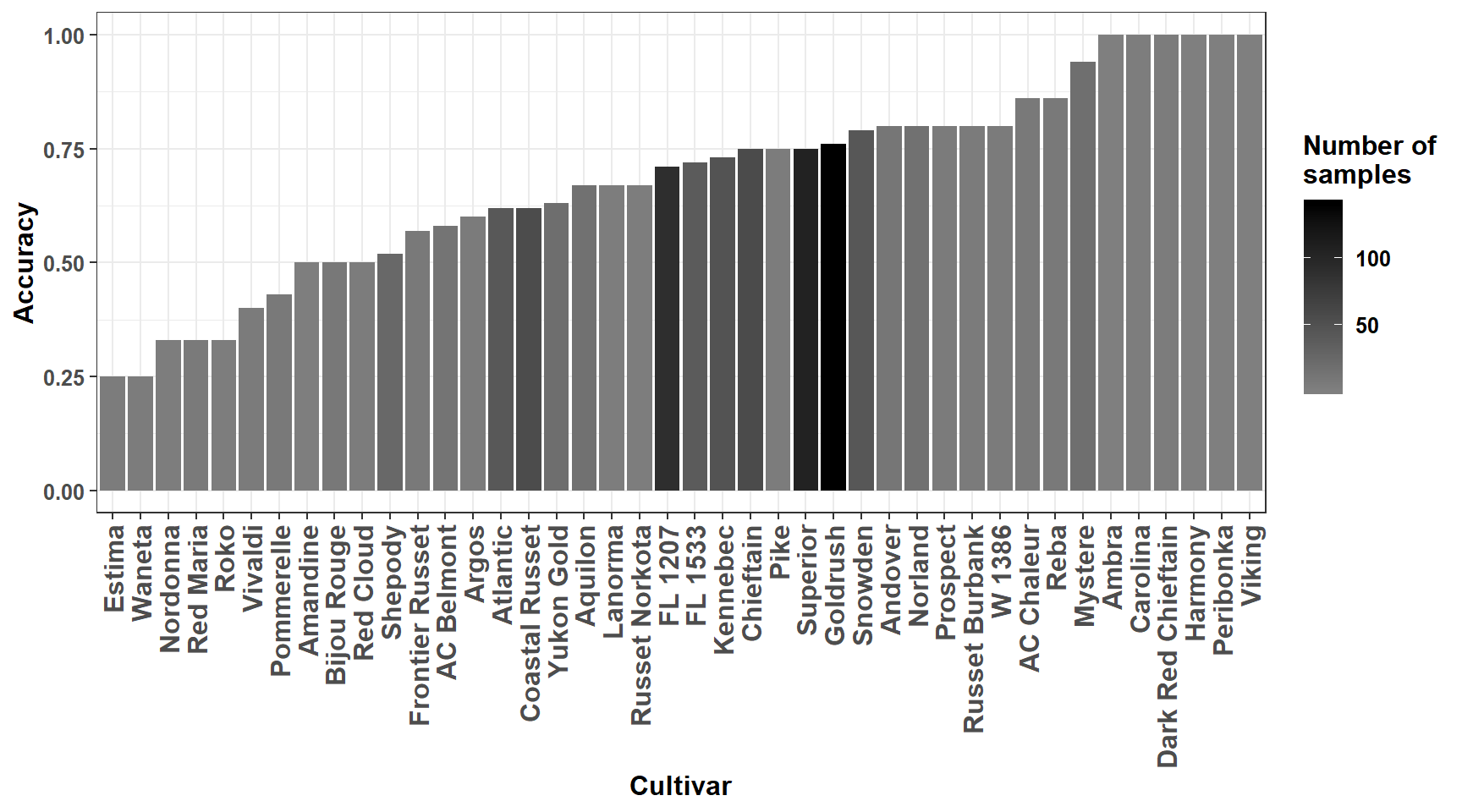
Figure 3.3: Predictive accuracy for cultivars.
3.7 Comparison with non-informative classification
The non-informative classification consists of an equal distribution of 50% successful and 50% unsuccessful classification cases (Swets J. A., 1988). We run the Chi-square homogenity test to compare predictive accuracy of the ..kknn.. model to this non-informative classification model.
##           Reference
## Prediction  HY  LY
##         HY 192 107
##         LY 141 405
# rf_clr_and_ionomicgroup model's classification
good_class <- cm$table[1,1]+cm$table[2,2] # HY or LY and correctly predicted
misclass <- cm$table[1,2]+cm$table[2,1] # wrong classification
ml_class <- c(good_class, misclass)
# Non-informative model (nim)
total <- sum(cm$table) # total number of samples
good_nim <- 0.50 * total
misclass_nim <- 0.50 * total
non_inf_model <- c(good_nim, misclass_nim)
# Matrix for chisquare test
m <- rbind(ml_class, non_inf_model)
m## [,1] [,2]
## ml_class 597.0 248.0
## non_inf_model 422.5 422.5##
## Pearson's Chi-squared test with Yates' continuity correction
##
## data: m
## X-squared = 74.422, df = 1, p-value < 2.2e-16The null hypothesis for a non-informative classification is rejected after the chi-square homogeneity test, the too small p-value denotes important difference between the models.
3.8 Nutritionally balanced compositions
We consider as True Negatives (TN) specimens for this study, observations of the training data set having a high yield (HY) and correctly predicted with the __k nearest neighbors__ model.
Let’s save prediction for training set.
tr_pred <- predict(kknn_)#, train_df %>% select(ml_col))
train_df <- bind_cols(dfml[split_index, ], pred_yield = tr_pred)Then, we compute clr centroids (means) for cultivars using True Negatives original (not scaled) clr values. These centroids (S3 Table of the article) could be used as provisional clr mean norms for cultivars. The standard deviations could also be computed. We considered all the TNs as norms. Cultivars Lamoka and Sifra had no true negative specimens.
## Adding missing grouping variables: `Cultivar`## # A tibble: 45 x 7
## Cultivar clr_N clr_P clr_K clr_Mg clr_Ca clr_Fv
## <chr> <dbl> <dbl> <dbl> <dbl> <dbl> <dbl>
## 1 AC Belmont 0.703 -2.12 0.622 -1.62 -1.07 3.49
## 2 AC Chaleur 0.704 -1.93 0.360 -1.55 -1.07 3.50
## 3 Amandine 0.519 -2.29 0.557 -1.62 -0.696 3.53
## 4 Ambra 0.713 -1.98 0.275 -1.39 -1.08 3.46
## 5 Andover 0.904 -2.20 0.743 -2.19 -0.850 3.60
## 6 Aquilon 0.810 -1.94 0.404 -1.83 -0.894 3.45
## 7 Argos 0.819 -1.75 0.402 -1.70 -1.13 3.36
## 8 Atlantic 0.775 -1.90 0.132 -1.50 -1.07 3.57
## 9 Bijou Rouge 0.962 -2.06 0.598 -2.16 -1.01 3.68
## 10 Carolina 0.595 -2.18 0.114 -1.32 -0.833 3.63
## # ... with 35 more rowsWe also save prediction for testing set.
te_pred <- predict(kknn_, test_df %>% select(ml_col))
test_df <- bind_cols(dfml[-split_index, ], pred_yield = te_pred)
And finally backup for the next chapter.