Chapter 4 Ionome perturbation concept

4.1 Objective

---

The objective of this chapter is to show the user a visual example of perturbation effect in a Simplex, and to develop a mathematical workflow useful to adjust the ionome of potato crops for diagnostic purpose.

Perturbation in compositional space plays the same role as translation plays in real space. The assumption is that some natural processes in nature can be interpreted as a change from one composition C1 to another C2 through the application of a perturbation:

p ⊕ C1 ===> C2.

The difference between a new observation and a closest healthy composition (closest true negative - TN) or reference composition can be back-transformed to the compositional space. The resulted vector is the perturbation vector.

Theoretically, a misbalanced composition could be balanced (translated into a healthy zone) using a perturbation operation. Using this concept, ionome of a new cultivar could be assigned to the cultivar sharing similar leaf composition, and where nutrient requirements have been already documented by fertilizer trials.

We used the testing set to display the effect of a perturbation on the whole simplex. We selected two elements (N and P) and simulated an increase of their initial (observed) clr values by 20% (theoretically). The observed (observation) and new clr vector (perturbation) were back transformed to N, P, K, Ca, Mg and Fv compositional space for comparison.

Secondly, the procedure used to rebalance a misbalanced composition is decribed. As explained at the end of the Chapter 3, we consider as True Negatives (TN) specimens (or healthy points) for this study, observations of the training set having a high yield (HY) and correctly predicted by the k nearest neighbors model.

---

4.2 Data set and useful libraries

We need package compositions for further clr back-transformation to compositional space. The package reshape will be used to melt an intermediate data frame.

library("tidyverse")
library("extrafont")
library('compositions')
library("reshape")

The previous train_df and test_df are loaded.

train_df = read_csv("output/train_df.csv")

## Parsed with column specification:
## cols(
##   NoEssai = col_double(),
##   NoBloc = col_double(),
##   NoTraitement = col_double(),
##   clr_N = col_double(),
##   clr_P = col_double(),
##   clr_K = col_double(),
##   clr_Ca = col_double(),
##   clr_Mg = col_double(),
##   clr_Fv = col_double(),
##   RendVendable = col_double(),
##   rv_cut = col_double(),
##   yieldClass = col_character(),
##   Maturity5 = col_character(),
##   Cultivar = col_character(),
##   pred_yield = col_character()
## )

test_df = read_csv("output/test_df.csv")

## Parsed with column specification:
## cols(
##   NoEssai = col_double(),
##   NoBloc = col_double(),
##   NoTraitement = col_double(),
##   clr_N = col_double(),
##   clr_P = col_double(),
##   clr_K = col_double(),
##   clr_Ca = col_double(),
##   clr_Mg = col_double(),
##   clr_Fv = col_double(),
##   RendVendable = col_double(),
##   rv_cut = col_double(),
##   yieldClass = col_character(),
##   Maturity5 = col_character(),
##   Cultivar = col_character(),
##   pred_yield = col_character()
## )

TNs = train_df %>% filter(yieldClass == 'HY' & pred_yield == 'HY')
clr_no = c("clr_N", "clr_P", "clr_K", "clr_Ca", "clr_Mg", "clr_Fv")

Filtrer train_df et test_df pour ne conserver que les observations ayant les cultivars correspondant dans les vrais négatifs, et seulement les déséquilibrés.

train_df <- train_df %>% filter(Cultivar %in% unique(TNs$Cultivar))
test_df <- test_df %>% filter(Cultivar %in% unique(TNs$Cultivar))

4.3 Euclidean distance from nutritionally balanced compositions

The chunk below activates the custom function used to compute Euclidean distance.

eucl_dist_f <- function(x, y) {
    sqrt(sum((x-y)^2))
}

For each imbalanced composition, we use the next loop to compute all the euclidean distances between all the compositions in “TNs” of the corresponding cultivar. The computation is possible even if the cultivar is unknown, the loop must just be updated. Here, the loop returns the smallest Euclidean distance stored in debal vector.

For train_df:

debal <- c()
debal_index <- c()
for (i in 1:nrow(train_df)) {
    clr_i <- as.numeric(train_df[i, clr_no])
    TNs_target <- TNs %>% filter(Cultivar == train_df$Cultivar[i]) %>% select(clr_no)
    eucl_dist <- apply(TNs_target, 1, function(x) eucl_dist_f(x = x, y = clr_i))
    debal_index[i] <- which.min(eucl_dist)
    debal[i] <- eucl_dist[debal_index[i]]
}
train_df$debal <- debal
train_df <- train_df %>% filter(debal != 0)
train_df %>% glimpse()

## Observations: 1,724
## Variables: 16
## $ NoEssai      <dbl> 1, 1, 1, 1, 1, 1, 1, 1, 1, 1, 4, 4, 4, 4, 4, 4, 4...
## $ NoBloc       <dbl> 1, 1, 1, 1, 2, 2, 2, 3, 3, 3, 1, 2, 2, 2, 2, 3, 3...
## $ NoTraitement <dbl> 1, 2, 3, 6, 1, 2, 8, 4, 5, 7, 1, 1, 2, 3, 4, 2, 3...
## $ clr_N        <dbl> 0.3321186, 0.4252302, 0.4453417, 0.4885647, 0.473...
## $ clr_P        <dbl> -2.518325, -2.394957, -2.365429, -2.525335, -2.28...
## $ clr_K        <dbl> 0.8379383, 1.1387291, 1.0112272, 0.9418880, 0.718...
## $ clr_Ca       <dbl> -0.4794688, -0.5154924, -0.7290838, -0.6426036, -...
## $ clr_Mg       <dbl> -1.639076, -2.346167, -1.990736, -1.763195, -1.69...
## $ clr_Fv       <dbl> 3.466813, 3.692658, 3.628680, 3.500681, 3.337752,...
## $ RendVendable <dbl> 18.944200, 40.351800, 33.037900, 41.016700, 15.11...
## $ rv_cut       <dbl> 41.33053, 41.33053, 41.33053, 41.33053, 41.33053,...
## $ yieldClass   <chr> "LY", "LY", "LY", "LY", "LY", "LY", "HY", "LY", "...
## $ Maturity5    <chr> "mid-season", "mid-season", "mid-season", "mid-se...
## $ Cultivar     <chr> "Goldrush", "Goldrush", "Goldrush", "Goldrush", "...
## $ pred_yield   <chr> "LY", "LY", "HY", "LY", "LY", "HY", "LY", "LY", "...
## $ debal        <dbl> 0.4859422, 0.3245021, 0.2126167, 0.2987338, 0.384...

For test_df:

debal <- c()
debal_index <- c()
for (i in 1:nrow(test_df)) {
    clr_i <- as.numeric(test_df[i, clr_no])
    TNs_target <- TNs %>% filter(Cultivar == test_df$Cultivar[i]) %>% select(clr_no)
    eucl_dist <- apply(TNs_target, 1, function(x) eucl_dist_f(x = x, y = clr_i))
    debal_index[i] <- which.min(eucl_dist)
    debal[i] <- eucl_dist[debal_index[i]]
}
test_df$debal <- debal
test_df <- test_df %>% filter(debal != 0)
test_df %>% glimpse()

## Observations: 803
## Variables: 16
## $ NoEssai      <dbl> 1, 1, 1, 1, 1, 1, 1, 1, 4, 4, 4, 4, 4, 5, 5, 5, 5...
## $ NoBloc       <dbl> 1, 1, 2, 2, 2, 3, 3, 3, 1, 1, 1, 1, 3, 1, 1, 1, 2...
## $ NoTraitement <dbl> 4, 5, 5, 6, 7, 1, 2, 8, 2, 3, 5, 6, 1, 2, 4, 5, 5...
## $ clr_N        <dbl> 0.3993264, 0.6519389, 0.5692523, 0.7251908, 0.507...
## $ clr_P        <dbl> -2.599180, -2.468221, -2.423432, -2.327678, -2.50...
## $ clr_K        <dbl> 0.7945826, 0.8242433, 0.7214698, 0.7597218, 0.676...
## $ clr_Ca       <dbl> -0.6220171, -0.7470790, -0.6610863, -0.6945233, -...
## $ clr_Mg       <dbl> -1.577529, -1.775074, -1.730285, -1.991205, -1.51...
## $ clr_Fv       <dbl> 3.604817, 3.514191, 3.524081, 3.528494, 3.430364,...
## $ RendVendable <dbl> 37.55050, 46.00890, 42.95690, 49.24620, 41.86690,...
## $ rv_cut       <dbl> 41.33053, 41.33053, 41.33053, 41.33053, 41.33053,...
## $ yieldClass   <chr> "LY", "HY", "HY", "HY", "HY", "LY", "LY", "HY", "...
## $ Maturity5    <chr> "mid-season", "mid-season", "mid-season", "mid-se...
## $ Cultivar     <chr> "Goldrush", "Goldrush", "Goldrush", "Goldrush", "...
## $ pred_yield   <chr> "HY", "HY", "LY", "LY", "LY", "LY", "HY", "LY", "...
## $ debal        <dbl> 0.48988609, 0.16712719, 0.23425051, 0.21198871, 0...

4.4 Perturbation effect of some elements on the whole

This subsection illustrates the principle that strictly positive data constrained to some whole are inherently related to each other. Changing a proportion (so, perturbation on some proportion(s)) inherently affects at least another proportion, because such data convey only relative information (Aitchison, 1982).

leaf_clr_o stands for original clr values of the tidded test set test_df.

# Compute (or select here) the clrs
leaf_clr_o <- test_df %>% select(clr_no)
#leaf_clr_o <- test_df %>% 
#  filter(debal >= quantile(train_df$debal, p = .75)) %>% 
#  select(clr_no)
summary(leaf_clr_o)

##      clr_N            clr_P            clr_K             clr_Ca        
##  Min.   :0.0000   Min.   :-3.159   Min.   :-0.3560   Min.   :-1.98953  
##  1st Qu.:0.6253   1st Qu.:-2.171   1st Qu.: 0.2671   1st Qu.:-1.16304  
##  Median :0.7282   Median :-2.005   Median : 0.4315   Median :-1.00005  
##  Mean   :0.7227   Mean   :-2.004   Mean   : 0.4567   Mean   :-1.00711  
##  3rd Qu.:0.8349   3rd Qu.:-1.838   3rd Qu.: 0.6078   3rd Qu.:-0.84266  
##  Max.   :1.2106   Max.   :-1.186   Max.   : 1.8047   Max.   : 0.06082  
##      clr_Mg            clr_Fv     
##  Min.   :-2.7207   Min.   :2.969  
##  1st Qu.:-1.9545   1st Qu.:3.472  
##  Median :-1.7108   Median :3.547  
##  Mean   :-1.7294   Mean   :3.561  
##  3rd Qu.:-1.5006   3rd Qu.:3.640  
##  Max.   :-0.6952   Max.   :4.167

Let’s perturb the original clr values for N and P.

# Perturb the original clrs
pert_col <- c(1, 2) # the column indices which is perturbed: clr_N and clr_K respectively
perturbation <- c(0.2, 0.2) # the amount added to the clr of the pert_col, same lenght as pert_col
leaf_clr_f <- leaf_clr_o
for (i in seq_along(pert_col)) {
  leaf_clr_f[, pert_col[i]] <- leaf_clr_f[, pert_col[i]] * (1 + perturbation[i])
}
summary(leaf_clr_f)

##      clr_N            clr_P            clr_K             clr_Ca        
##  Min.   :0.0000   Min.   :-3.791   Min.   :-0.3560   Min.   :-1.98953  
##  1st Qu.:0.7503   1st Qu.:-2.605   1st Qu.: 0.2671   1st Qu.:-1.16304  
##  Median :0.8739   Median :-2.406   Median : 0.4315   Median :-1.00005  
##  Mean   :0.8672   Mean   :-2.404   Mean   : 0.4567   Mean   :-1.00711  
##  3rd Qu.:1.0019   3rd Qu.:-2.206   3rd Qu.: 0.6078   3rd Qu.:-0.84266  
##  Max.   :1.4528   Max.   :-1.423   Max.   : 1.8047   Max.   : 0.06082  
##      clr_Mg            clr_Fv     
##  Min.   :-2.7207   Min.   :2.969  
##  1st Qu.:-1.9545   1st Qu.:3.472  
##  Median :-1.7108   Median :3.547  
##  Mean   :-1.7294   Mean   :3.561  
##  3rd Qu.:-1.5006   3rd Qu.:3.640  
##  Max.   :-0.6952   Max.   :4.167

The next one transforms clrs (original and perturbed clrs) back to compositions.

# From clrs to compositions
leaf_o <- apply(leaf_clr_o, 1, function(x) exp(x) / sum(exp(x))) %>% t()
leaf_f <- apply(leaf_clr_f, 1, function(x) exp(x) / sum(exp(x))) %>% t()

Then, we plot the original and perturbed ionomes to check a general tendency. Observation column plots the original “N”, “P”, “K”, “Ca”, “Mg” and “Fv” compositions, Perturbation represents new compositions after perturbation and Difference column stands for perturbation occured in the Observation to yied new compositions. Data are tidded before.

rshleaf_o <- melt(data.frame(leaf_o)) %>% mutate(vector = rep("Observation", nrow(.)))

## Using  as id variables

rshleaf_f <- melt(data.frame(leaf_f)) %>% mutate(vector = rep("Perturbation", nrow(.)))

## Using  as id variables

rshdf <- bind_rows(rshleaf_o, rshleaf_f)
rshdf$is_perturbed <- ifelse(rshdf$variable %in% colnames(leaf_o[, pert_col]), 
                          "Perturbed", "Not perturbed")

rshdf$variable <- sub(pattern = "clr_", replacement = "", x = rshdf$variable, fixed = TRUE) %>% 
  fct_relevel("N", "P", "K", "Ca", "Mg", "Fv")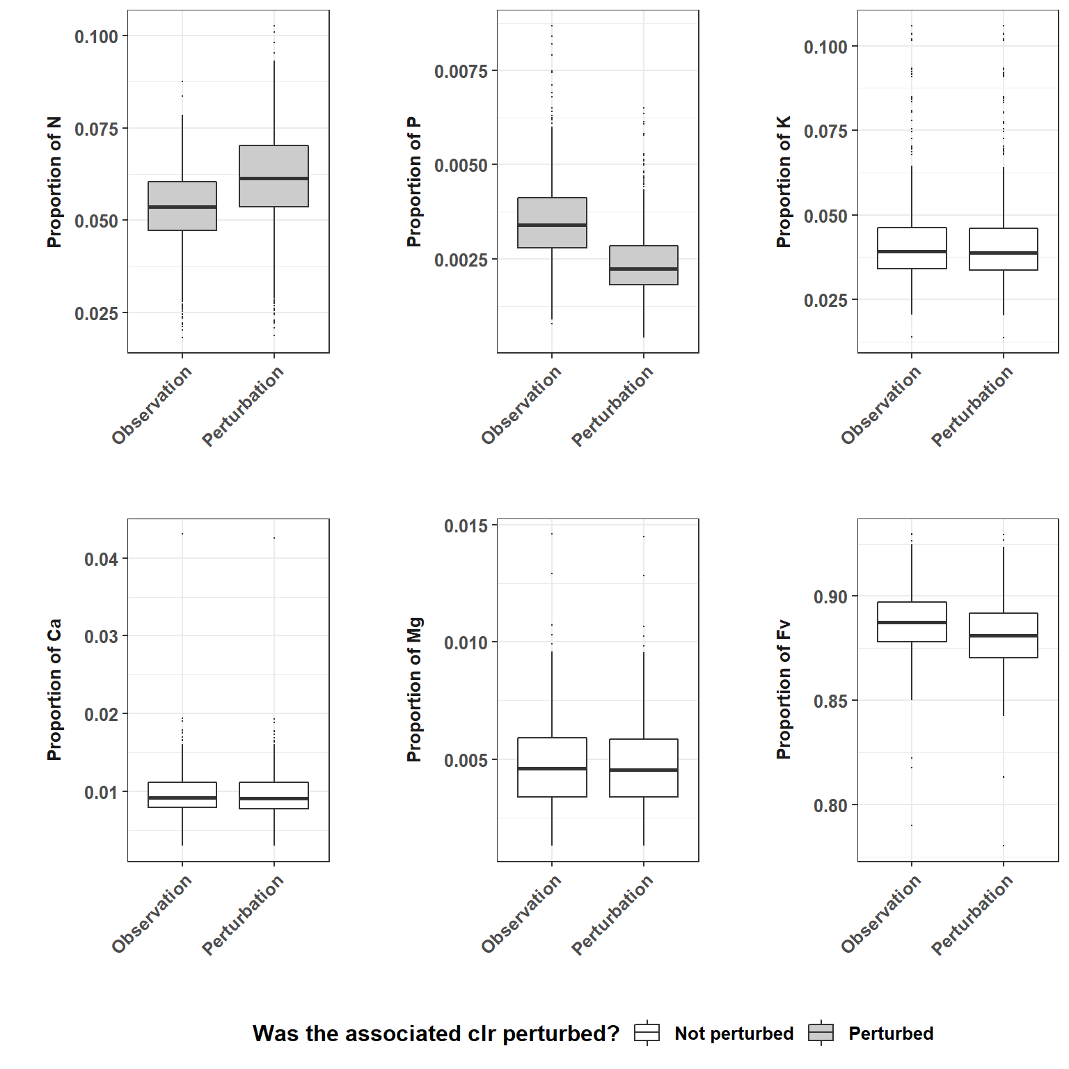

Figure 4.1: Perturbation effect of some elements on the whole.

All the components change when the clr of a single component is offset. The components whose clr has been perturbed obviously change the most (2-Perturbation). The component whose clr is the highest (generally Fv) compensate most of the perturbation. Although P clr values have been increased, P proportion decreased globally for the new equilibrium of the simplex.

4.5 Rebalancing a misbalanced sample by perturbation

Let’s suppose that we got this point selected at random in imbalanced or misbalanced specimens.

set.seed(92559) 
imbalanced <- train_df[sample(nrow(train_df), 1), ]
t(imbalanced)

##              [,1]        
## NoEssai      "412"       
## NoBloc       "1"         
## NoTraitement "9"         
## clr_N        "0.7735603" 
## clr_P        "-2.464426" 
## clr_K        "0.5688289" 
## clr_Ca       "-1.034959" 
## clr_Mg       "-1.660053" 
## clr_Fv       "3.817049"  
## RendVendable "34.74147"  
## rv_cut       "41.33053"  
## yieldClass   "LY"        
## Maturity5    "mid-season"
## Cultivar     "Goldrush"  
## pred_yield   "LY"        
## debal        "0.2208642"

Or even, we could rather use the most imbalanced occurrence, why not !

imbalanced <- train_df[which.max(train_df$debal), ]
misbalanced <- imbalanced # copy
t(misbalanced)

##              [,1]              
## NoEssai      "200"             
## NoBloc       "1"               
## NoTraitement "2"               
## clr_N        "0.957698"        
## clr_P        "-1.83199"        
## clr_K        "-0.04637332"     
## clr_Ca       "0.4678508"       
## clr_Mg       "-2.247862"       
## clr_Fv       "2.700677"        
## RendVendable "30.37194"        
## rv_cut       "32.6"            
## yieldClass   "LY"              
## Maturity5    "early mid-season"
## Cultivar     "Superior"        
## pred_yield   "LY"              
## debal        "1.345815"

How could we rebalance it? The first step is to find the closest balanced point in the TNs of the corresponding cultivar. Let’s re-compute its Euclidean distances from TNs and identify the TNs’ sample from which the distance is minimum.

misbalanced <- misbalanced[clr_no]
eucl_dist_misbal <- apply(TNs %>% filter(Cultivar == imbalanced$Cultivar) %>% select(clr_no), 
                          1, function(x) eucl_dist_f(x = x, y = misbalanced))

index_misbal <- which.min(t(data.frame(eucl_dist_misbal))) 
index_misbal # return the index of the sample

## [1] 50

The closest healthy sample is the one which index is 50 in TNs charing the same cultivar with the new sample. Using this index we could refind the minimum imbalance index value computed.

(misbal <- eucl_dist_misbal[index_misbal])

## [1] 1.345815

The Euclidean distance matches with the corresponding debal value: imbalanced$debal[1] = 1.3458148. The closest point in the TNs subset is this one:

target_TNs <- TNs %>% 
  filter(Cultivar == imbalanced$Cultivar)
closest <- target_TNs[index_misbal, ]
t(closest)

##              [,1]              
## NoEssai      "71"              
## NoBloc       "3"               
## NoTraitement "5"               
## clr_N        "0.5576154"       
## clr_P        "-2.078376"       
## clr_K        "0.4710692"       
## clr_Ca       "-0.3762287"      
## clr_Mg       "-2.022806"       
## clr_Fv       "3.448726"        
## RendVendable "37.56831"        
## rv_cut       "32.6"            
## yieldClass   "HY"              
## Maturity5    "early mid-season"
## Cultivar     "Superior"        
## pred_yield   "HY"

Note that Cultivar of the misbalanced and the closest healthy composition are the same. We compute the clr difference between the closest and the misbalanced points.

closest = closest[clr_no]
clr_diff = closest - misbalanced
t(clr_diff)

##              [,1]
## clr_N  -0.4000826
## clr_P  -0.2463863
## clr_K   0.5174425
## clr_Ca -0.8440794
## clr_Mg  0.2250562
## clr_Fv  0.7480496

The perturbation vector is that clr difference back-transformed to leaf compositional space.

comp_names <- c("N", "P", "K", "Ca", "Mg", "Fv")
perturbation_vector <- clrInv(clr_diff)
names(perturbation_vector) <- comp_names
t(perturbation_vector)

##    [,1]      
## N  0.09679140
## P  0.11287200
## K  0.24227737
## Ca 0.06208853
## Mg 0.18085523
## Fv 0.30511547
## attr(,"class")
## [1] acomp

Next, we should compute the corresponding compositions of the clr coordinates of the misbalanced point, as well as the closest TN point. The vectors could be gathered in a table made up of perturbation vector, misbalanced composition and the closest reference sample (pmc).

misbal_comp <- clrInv(misbalanced)
names(misbal_comp) <- comp_names

closest_comp <- clrInv(closest)
names(closest_comp) <- comp_names

pmc = rbind(perturbation_vector, misbal_comp, closest_comp)
rownames(pmc) = c("perturbation_vector","misbal_comp","closest_comp")
pmc

##                             N           P         K         Ca        Mg
## perturbation_vector 0.0967914 0.112872002 0.2422774 0.06208853 0.1808552
## misbal_comp         0.1282805 0.007881602 0.0470000 0.07860000 0.0052000
## closest_comp        0.0488500 0.003500000 0.0448000 0.01920000 0.0037000
##                            Fv
## perturbation_vector 0.3051155
## misbal_comp         0.7330379
## closest_comp        0.8799500

We could even check that the simplex is closed to 1 for each vector.

sum(perturbation_vector); sum(misbal_comp); sum(closest_comp)

## [1] 1

## [1] 1

## [1] 1

The closest composition minus the misbalanced composition should return the perturbation vector.

print(closest_comp - misbal_comp)

##      N         P        K         Ca         Mg        Fv       
## [1,] 0.0967914 0.112872 0.2422774 0.06208853 0.1808552 0.3051155
## attr(,"class")
## [1] acomp

print(perturbation_vector) # for comparison

##      N         P        K         Ca         Mg        Fv       
## [1,] 0.0967914 0.112872 0.2422774 0.06208853 0.1808552 0.3051155
## attr(,"class")
## [1] acomp

Or even, perturb the misbalanced point by the perturbation vector, you should obtain the closest TN point:

print(misbal_comp + perturbation_vector) # perturbation

##      N       P      K      Ca     Mg     Fv     
## [1,] 0.04885 0.0035 0.0448 0.0192 0.0037 0.87995
## attr(,"class")
## [1] acomp

print(closest_comp)                      # for comparison

##      N       P      K      Ca     Mg     Fv     
## [1,] 0.04885 0.0035 0.0448 0.0192 0.0037 0.87995
## attr(,"class")
## [1] acomp

So, the assumption is true. The next codes show the concept using dots plots and histograms for each vector. A data frame is tidded for ggplot. Visualization is better with histograms.

df <- data.frame(rbind(misbalanced, closest, clr_diff),
                 vectors = factor(c("Observation", "Reference", "Perturbation")))
df$vectors <- df$vectors %>% fct_relevel("Observation", "Reference", "Perturbation")
dfreshape <- melt(df) # reshapes df for ggplot

## Using vectors as id variables

dfreshape <- melt(df)

## Using vectors as id variables

dfreshape$variable <- sub(pattern = "clr_", replacement = "", x = dfreshape$variable, fixed = TRUE) %>% 
  fct_relevel("N", "P", "K", "Ca", "Mg", "Fv")

ggplot(data = dfreshape, aes(x = value, y = vectors, colour = vectors)) +
    geom_point() +
    facet_wrap(~ variable, scales = "free_x") +
    labs(x='Nutrient clr coordinate', y ='') +
    theme(text=element_text(family="Arial", face="bold", size=12)) +
    theme_bw()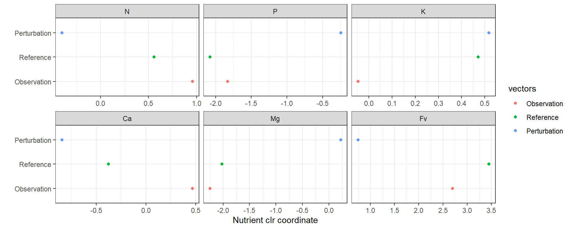

Figure 4.2: Perturbation vector computation example dotplot using the most imbalanced foliar sample.

ggsave("images/perturb_dotplot.tiff",  width = 7, height = 3)

g1 <- ggplot(data = dfreshape, aes(x = variable, y = value, fill = vectors)) +
    geom_bar(aes(fill = vectors), stat = "identity", position = position_dodge()) +
    coord_flip() + theme_bw() +
    ylab("Nutrients clr coordinates") + xlab("Diagnostic nutrients") +
    theme(legend.title = element_blank()) +
    theme(text = element_text(family = "Arial", face = "bold", size = 12))
g1 + scale_fill_discrete(breaks = c("Observation","Reference","Perturbation")) +
    scale_fill_manual(values=c("grey50", "black", "grey80"))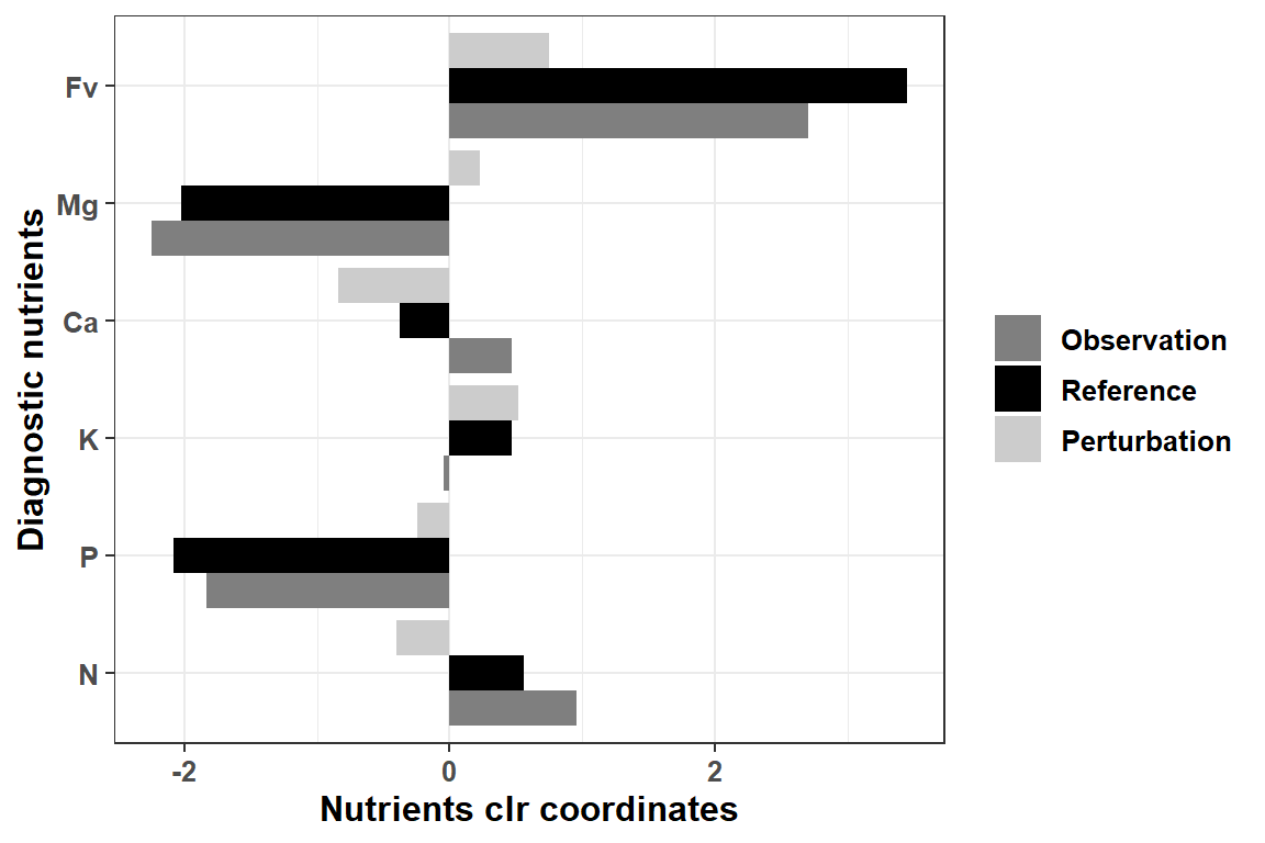

Figure 4.3: Perturbation vector computation example barplot using the most imbalanced foliar sample.

ggsave("images/perturb_barplot.tiff",  width = 6, height = 4)