Chapter 4 Perturbation vector theory
4.1 Objective
The objective of this chapter is to develop a mathematical workflow useful to adjust the ionome of potato crops for diagnostic purpose. Perturbation in compositional space plays the same role as translation plays in real space. Some natural processes in nature can be interpreted as a change from one composition C1 to another C2 through the application of a perturbation:
p ⊕ C1 ===> C2.
The difference between a new observation and the closest healthy composition (closest TN) can be back-transformed to the compositional space. The obtained vector is the perturbation vector. Theoretically, a misbalanced composition could be balanced (translated into a healthy zone) using a perturbation vector. Also, ionome of a new cultivar could be assigned to the closest healthy sample’s cultivar, where nutrient requirements have been already documented by fertilizer trials.
I compute a dissimilarity (or imbalance) index using the true negative clr as references for cultivars. Then, I describe the procedure used to rebalance a misbalanced composition.
4.2 Data set and useful libraries
We need package compositions for further clr back-transformation to compositional space. The package reshape will be used to melt an intermediate data frame. As explained at the end of the Chapter 3, I consider as True Negatives (TN) specimens (or healthy points) for this study, observations of the training data set having a high yield (HY) and correctly predicted by the random forest model.
library("tidyverse")
library("extrafont")
library('compositions')
library("reshape")
train_df = read_csv("output/train_df.csv")train_df$Cultivar = factor(train_df$Cultivar)
TNs = train_df %>%
filter(yieldClass == 'HY' & pred_yield == 'HY')
clrNo = c("clrN", "clrP", "clrK", "clrCa", "clrMg", "clrFv") # for simplicity4.3 Dissimilarity index between compositions
The first step is to compute a dissimilarity index according to the distance from the closest healthy point (the closest TN). I use the Aitchison distance (multivariate Euclidean distance) between clr composition as the dissimilarity index. The chunk below shows the custom function used to compute euclidean distance.
eucl_dist_f <- function(x, y) {
    sqrt(sum((x-y)^2))
}
For each unbalanced composition, I use the next loop to compute all the euclidean distances between all the compositions in “TNs” of the corresponding group. The computation is possible even if the ionomics groups is unknown. The loop returns the smallest Euclidean distance as the unbalanced index of that composition. The computed debalance (or imbalance) index is stored by a new vector debal.
debal <- c()
debal_index <- c()
for (i in 1:nrow(train_df)) {
    clr_i <- as.numeric(train_df[i, clrNo])
    eucl_dist <- apply(TNs %>% filter(Cultivar == train_df$Cultivar[i]) %>% select(clrNo), #
                       1, function(x) eucl_dist_f(x=x, y=clr_i))
    debal_index[i] <- which.min(eucl_dist)
    debal[i] <- eucl_dist[debal_index[i]]
}
train_df$debal <- debal
train_df %>% glimpse()
## Observations: 2,537
## Variables: 16
## $ NoEssai <dbl> 1, 1, 1, 1, 1, 1, 1, 1, 1, 1, 1, 1, 1, 1, 1, 1, 1...
## $ NoBloc <dbl> 1, 1, 1, 1, 1, 1, 2, 2, 2, 2, 2, 3, 3, 3, 3, 3, 3...
## $ NoTraitement <dbl> 1, 2, 4, 6, 7, 8, 2, 3, 4, 6, 7, 1, 2, 4, 6, 7, 8...
## $ clrN <dbl> 0.3321186, 0.4252302, 0.3993264, 0.4885647, 0.720...
## $ clrP <dbl> -2.518325, -2.394957, -2.599180, -2.525335, -2.30...
## $ clrK <dbl> 0.8379383, 1.1387291, 0.7945826, 0.9418880, 0.720...
## $ clrMg <dbl> -0.4794688, -0.5154924, -0.6220171, -0.6426036, -...
## $ clrCa <dbl> -1.639076, -2.346167, -1.577529, -1.763195, -1.70...
## $ clrFv <dbl> 3.466813, 3.692658, 3.604817, 3.500681, 3.432323,...
## $ RendVendable <dbl> 18.94420, 40.35180, 37.55050, 41.01670, 46.79370,...
## $ rv_cut <dbl> 41.33053, 41.33053, 41.33053, 41.33053, 41.33053,...
## $ yieldClass <chr> "LY", "LY", "LY", "LY", "HY", "HY", "LY", "HY", "...
## $ Cultivar <fct> Goldrush, Goldrush, Goldrush, Goldrush, Goldrush,...
## $ Maturity5 <chr> "mid-season", "mid-season", "mid-season", "mid-se...
## $ pred_yield <chr> "LY", "LY", "LY", "LY", "HY", "HY", "LY", "HY", "...
## $ debal <dbl> 0.2915435, 0.3247296, 0.2628167, 0.2987338, 0.000...simplement pour apprécier la corrélation entre indice de debalancement et rendement
Add regression line, correlation coefficient and equantions of the fitted line. Key functions: > stat_smooth() [ggplot2] > stat_cor() [ggpubr] > stat_poly_eq()[ggpmisc]
library("ggpubr")
library("ggpmisc")
# Polynomial regression. Show equation and adjusted R2
data <- train_df %>% filter(debal != 0); x = data$debal; y = data$RendVendable
formula <- y ~ poly(x, 2)#, raw = TRUE)
p <- ggplot(data = data, aes(x = debal, y = RendVendable)) +
geom_point() +
geom_smooth(formula = formula) +
stat_poly_eq(
aes(label = paste(..eq.label.., ..adj.rr.label.., sep = "~~~~")),
formula = formula, parse = TRUE, label.x = 0.50
)
p## `geom_smooth()` using method = 'gam' and formula 'y ~ s(x, bs = "cs")'
Fin appréciation.
4.4 Rebalancing a misbalanced sample by perturbation
Let’s suppose that we got this point selected at random in unbalanced specimens.
set.seed(932559)
unbalanced <- subset(train_df, debal !=0)
unbalanced <- unbalanced[sample(nrow(unbalanced), 1), ]
t(unbalanced)
## [,1]
## NoEssai "355"
## NoBloc "1"
## NoTraitement "2"
## clrN "0.8015935"
## clrP "-2.00352"
## clrK "0.1670366"
## clrMg "-0.8453153"
## clrCa "-1.563568"
## clrFv "3.443773"
## RendVendable "33.14916"
## rv_cut "33.63704"
## yieldClass "LY"
## Cultivar "Mystere"
## Maturity5 "late"
## pred_yield "LY"
## debal "0.2125451"Or even, we could rather use the most unbalanced occurrence, why not !
unbalanced <- subset(train_df, debal !=0)
unbalanced <- unbalanced[which.max(unbalanced$debal), ]
misbalanced <- unbalanced # copy
t(misbalanced)
## [,1]
## NoEssai "200"
## NoBloc "1"
## NoTraitement "2"
## clrN "0.957698"
## clrP "-1.83199"
## clrK "-0.04637332"
## clrMg "0.4678508"
## clrCa "-2.247862"
## clrFv "2.700677"
## RendVendable "30.37194"
## rv_cut "32.6"
## yieldClass "LY"
## Cultivar "Superior"
## Maturity5 "early mid-season"
## pred_yield "LY"
## debal "1.256154"How could we rebalance it? The first step is to find in TNs of the corresponding cultivar the closest balanced point. Let’s re-compute its Euclidean distances from TNs and identify the sample from which the distance is minimum.
misbalanced <- misbalanced[clrNo]
eucl_dist_misbal <- apply(TNs[, clrNo], 1, function(x) eucl_dist_f(x = x, y = misbalanced))
index_misbal <- which.min(t(data.frame(eucl_dist_misbal)))
index_misbal # return the index of the sample
## [1] 610The closest healthy sample is the one which index is 610. Using this index we could refind the imbalance index value (debal) of the misbalanced sample for check.
(misbal = eucl_dist_misbal[index_misbal])## [1] 1.256154The Euclidean distance matches with the corresponding debal value: unbalanced$debal[1] = 1.2561535.
The closest point in the TNs subset is this one:
closest <- TNs[index_misbal, ]
t(closest)
## [,1]
## NoEssai "196"
## NoBloc "3"
## NoTraitement "6"
## clrN "0.6219769"
## clrP "-2.544439"
## clrK "0.3293346"
## clrMg "0.02902074"
## clrCa "-1.635584"
## clrFv "3.199691"
## RendVendable "41.2204"
## rv_cut "32.6"
## yieldClass "HY"
## Cultivar "Superior"
## Maturity5 "early mid-season"
## pred_yield "HY"Note that Cultivar of the misbalanced and the closest healthy composition are the same. I compute the clr difference between the closest and the misbalanced points.
closest = closest[clrNo]
clr_diff = closest - misbalanced
t(clr_diff)
## [,1]
## clrN -0.3357211
## clrP -0.7124496
## clrK 0.3757079
## clrCa 0.6122787
## clrMg -0.4388300
## clrFv 0.4990141The perturbation vector is that clr difference back-transformed to leaf compositional space.
comp_names <- c("N", "P", "K", "Ca", "Mg", "Fv")
perturbation_vector <- clrInv(clr_diff)
names(perturbation_vector) <- comp_names
t(perturbation_vector)
## [,1]
## N 0.10515492
## P 0.07214704
## K 0.21419006
## Ca 0.27135681
## Mg 0.09485276
## Fv 0.24229840
## attr(,"class")
## [1] acompNext, we should compute the compositions of the clr coordinates of the misbalanced point, as well as the closest TN point. The vectors could be gathered in a table made up of perturbation vector, misbalanced composition and the closest reference sample (pmc).
misbal_comp <- clrInv(misbalanced)
names(misbal_comp) <- comp_names

closest_comp <- clrInv(closest)
names(closest_comp) <- comp_names

pmc = rbind(perturbation_vector, misbal_comp, closest_comp)
rownames(pmc) = c("perturbation_vector","misbal_comp","closest_comp")
pmc
## N P K Ca Mg
## perturbation_vector 0.10515492 0.072147042 0.2141901 0.2713568 0.09485276
## misbal_comp 0.12828046 0.007881602 0.0470000 0.0052000 0.07860000
## closest_comp 0.06405025 0.002700000 0.0478000 0.0067000 0.03540000
## Fv
## perturbation_vector 0.2422984
## misbal_comp 0.7330379
## closest_comp 0.8433497We could even check that the simplex is closed to 1 for each vector.
sum(perturbation_vector); sum(misbal_comp); sum(closest_comp)## [1] 1## [1] 1## [1] 1The closest composition minus the misbalanced composition should return the perturbation vector.
print(closest_comp - misbal_comp) # soustraction## N P K Ca Mg Fv
## [1,] 0.1051549 0.07214704 0.2141901 0.2713568 0.09485276 0.2422984
## attr(,"class")
## [1] acompprint(perturbation_vector) # for comparison## N P K Ca Mg Fv
## [1,] 0.1051549 0.07214704 0.2141901 0.2713568 0.09485276 0.2422984
## attr(,"class")
## [1] acompOr even, perturb the misbalanced point by the perturbation vector, you should obtain the closest TN point:
print(misbal_comp + perturbation_vector) # perturbation## N P K Ca Mg Fv
## [1,] 0.06405025 0.0027 0.0478 0.0067 0.0354 0.8433497
## attr(,"class")
## [1] acompprint(closest_comp) # for comparison## N P K Ca Mg Fv
## [1,] 0.06405025 0.0027 0.0478 0.0067 0.0354 0.8433497
## attr(,"class")
## [1] acompSo, the assumption is true. The next codes show the concept using plots. I aranged a data frame for ggplot.
df = data.frame(rbind(misbalanced, closest, clr_diff))
vectors = c("observation", "reference", "perturbation")
df$vectors = factor(vectors)
dfreshape = melt(df) # reshapes df for ggplot
## Using vectors as id variablesdfreshape## vectors variable value
## 1 observation clrN 0.95769802
## 2 reference clrN 0.62197688
## 3 perturbation clrN -0.33572114
## 4 observation clrP -1.83198972
## 5 reference clrP -2.54443931
## 6 perturbation clrP -0.71244958
## 7 observation clrK -0.04637332
## 8 reference clrK 0.32933456
## 9 perturbation clrK 0.37570788
## 10 observation clrCa -2.24786229
## 11 reference clrCa -1.63558355
## 12 perturbation clrCa 0.61227874
## 13 observation clrMg 0.46785078
## 14 reference clrMg 0.02902074
## 15 perturbation clrMg -0.43883004
## 16 observation clrFv 2.70067654
## 17 reference clrFv 3.19969068
## 18 perturbation clrFv 0.49901414The next two chunks plot with dots and histograms for each vector. Visualization is better with histograms.
ggplot(data = dfreshape, aes(x = value, y = vectors, colour = vectors)) +
    geom_point() +
    facet_wrap(~ variable, scales = "free_x") +
    labs(x='clr coordinate', y ='') +
    theme(text=element_text(family="Arial", face="bold", size=12))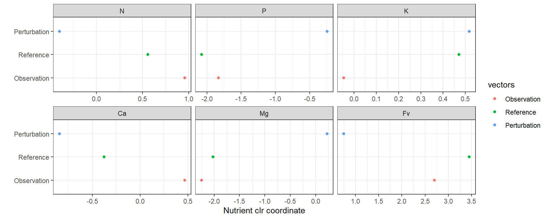
Figure 4.1: Perturbation vector computation example dotplot using the most imbalanced foliar sample.
ggsave("images/perturb_dotplot.tiff", width = 6, height = 3)ggplot(data=dfreshape, aes(x=variable, y=value, fill=vectors)) +
geom_bar(stat="identity", position=position_dodge()) +
coord_flip() +
theme_bw() +
theme(legend.title=element_blank()) +
theme(text=element_text(family="Arial", face="bold", size=12))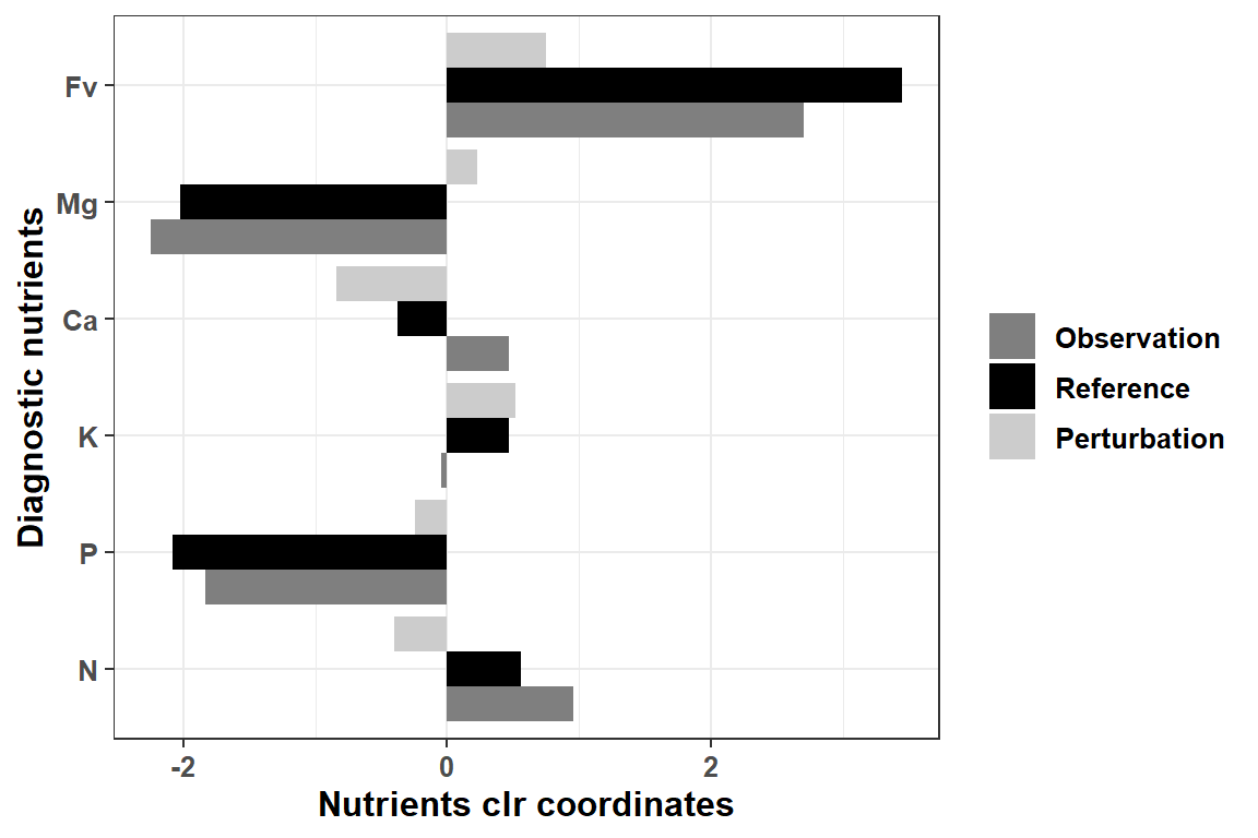
Figure 4.2: Perturbation vector computation example barplot using the most imbalanced foliar sample.
ggsave("images/perturb_barplot.tiff", width = 6, height = 3)